Searching, please wait
 Print
Print
 Add to library
 Discuss this article
Ochoa Sangrador C, Molina Arias M. Evaluación de la precisión de las pruebas diagnósticas (2). Variables continuas. Evid Pediatr. 2017;13:45.
In previous articles in this series, we have addressed how to assess the validity of a diagnostic test. We have also reviewed how to assess its accuracy or reliability. To date, we have discussed the methods used to measure the accuracy of discrete data, nominal (kappa statistic) and ordinal (weighted kappa statistic). In this article, we will broach the methods that apply to continuous data: the within-subject standard deviation, the intraclass correlation coefficient and the Bland and Altman method.
When the result of a test is measured on a continuous scale, we can estimate the measurement error by calculating the variability that exists between repeated measurements in the same subjects. The parameter that best reflects such variability is the within-subject standard deviation (excluding the variability observed between subjects). To calculate it, we need a set of subjects to undergo at least two measurements each. Table 1 presents the results of performing two repeated transcutaneous bilirubin measurements in newborns with jaundice.1 The within-subject standard deviation can be calculated easily using software that performs analysis of variance (ANOVA). ANOVA breaks down the variation present in the set of measurements (estimated based on the squared differences of each value and the mean of all subjects) into several components: the variation in measurements taken in different subjects (between rows in Table 1) and the variation in the residuals, which in one-way ANOVA corresponds to the variation in the measurements taken in each subject (between columns in Table 1).
Table 1. Results of two repeated transcutaneous bilirubin measurements (Jaundice-Meter 101, Minolta Air Shields) in the anterior surface of the thorax in 20 newborns with jaundice. Data retrieved from a larger study.3 Show/hide
Table 2 shows the ANOVA for the data in Table 1. The parameter called mean square of the residuals (MSr) is the residual or within-subject variance (which depends on the differences between repeated measures in each subject). If we take the square root of the MSr, we obtain the within-subject standard deviation (sw). The sw can also be calculated using the results of ANOVA in designs with more than two measurements per subject.
Table 2. One-way analysis of variance for the data in Table 1. Show/hide
We can use the sw to quantify the margin of error in our measurements. Thus, we can estimate that the difference between a specific measurement and the true value will not be greater than 1.96 times the sw in 95% of observations (assuming that the data follow a normal distribution, 95% of the measurements will be contained in the interval formed by the actual value plus and minus 1.96 times the standard deviation). It also allows us to estimate that the difference between two measurements for the same subject will not exceed 2.77 times the sw in 95% of observations.2,3 In our example, the sw is 0.54 (square root of 0.3), so the estimated difference from the true value would be of less than 1.05 (1.96 × 0.54) and the difference between two measurements would be of less than 1.49 (2.77 × 0.54).
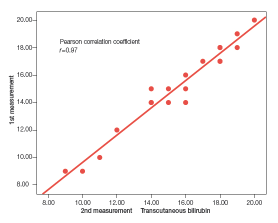
If only two measurements are taken per subject, the most intuitive way to compare them is to plot measurement pairs in a scatter diagram, assess whether there is a linear association between them, and calculate the corresponding correlation coefficient. Figure 1 shows the scatter diagram for the data in Table 1. The Pearson correlation coefficient (r) for these data is 0.97 (the closer r is to 1, the stronger the correlation).
Figure 1. Scatter plot and linear correlation for the data in Table 1. Show/hide
However, the presence of a strong linear association with a high correlation coefficient does not prove a strong agreement between the measurements, but only that the points in the plot fit a straight line well. The correlation coefficient is largely dependent on inter-subject variability and thus changes substantially based on the characteristics of the sample for which it is calculated, and is especially sensitive to the presence of extreme values. If one of the measurements is systematically greater than the other, the correlation coefficient will be very high, despite the fact that the measurements never agree. These pitfalls can be avoiding by using the intraclass correlation coefficient.
The intraclass correlation coefficient (ICC) estimates the agreement between two or more repeated measurements. The calculation of the ICC is based on a repeated measures ANOVA model, applying different formulas based on the design and objectives of the study.4 In the simplest scenario, we would estimate the variability of the measurements without taking into account the variability contributed by different raters (one-way random effects model). Choosing this model, and using the results of ANOVA, we can calculate the ICC with the following formula:
$$CCI=\frac{CMp-CMr}{CMp+(k-1)CMr},$$where k stands for the number of observations per subject, MSp for the mean square between patients (which depends on the differences in measurements between subjects) and MSr for the mean square of the residuals (which depends on the differences between repeated measurements in each subject).
Using the data of the ANOVA in Table 2, the ICC will be:
$$CCI=\frac{19,55-0,30}{19,55+(2-1)0,30}= 0,96.$$In our example, there is hardly any difference between the ICC and the Pearson correlation coefficient (r). If the ICC were much smaller than r, one would assume that there is a systematic change between one measurement and the other, which may result from a learning effect. In this case, the measurements would not have been made under the same circumstances, so the conditions required for performing a reliability analysis would not be met.5
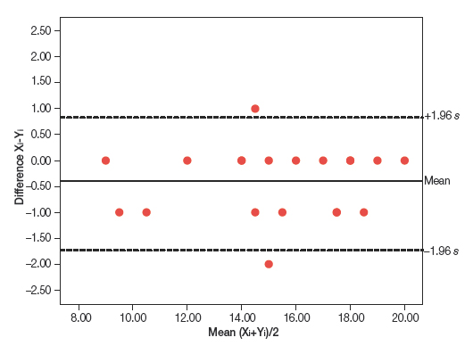
An alternative approach to analysing the agreement between two repeated observations measured on a continuous scale is the graphical method described by Bland and Altman.6 It consists of plotting the difference of each pair of measurements against the mean of the two measurements (Figure 2). The points tend to cluster around zero in the axis representing the difference between paired measurements, and the greater the dispersion around zero, the lesser the agreement between the two measurement methods. One possible way to assess agreement is to draw horizontal lines at the level of the maximum difference that would be acceptable from a clinical standpoint, and check whether the points, or most of the points, are grouped between these two horizontal lines. An alternative approach is to estimate the standard deviation of the differences and the interval in which we would expect to find 95% of them.
Figure 2. Bland and Altman method applied to the data in Table 1. Show/hide
This method can also be used to assess the magnitude of the differences and their association with the magnitude of the measurement. When the variability in the measurements is not constant, but changes as the magnitude of the measurement increases or decreases, the calculation becomes complicated.7 If there is a significant correlation between the differences and the means, the variability will not be constant (there may be an acceptable agreement in a specific value interval, but not in others). In this case, a logarithmic transformation of the data can be attempted, or else the variability can be analysed separately for various data intervals, although we should always hold reservations about the validity of measurements in these intervals.
Ochoa Sangrador C, Molina Arias M. Evaluación de la precisión de las pruebas diagnósticas (2). Variables continuas. Evid Pediatr. 2017;13:45.


 Full Article
 PDF
PDF Versión española